Appendix D – Navigation

Every EPCSAR member who expects to participate in SAR field activities or in overhead planning and operations must be proficient with use of map and compass. Use of map and compass is essential for efficient wilderness navigation, communicating positions, assessing terrain, defining search boundaries, and defining search strategies. Accomplishing these tasks involves a few basic skills with map and compass together with experience in their application. The purpose of this chapter is to explain these basic skills.

This chapter also covers use of Global Positioning System (GPS) receivers, which offer a very accurate means of land navigation. While familiarity with use of GPS receivers is strongly encouraged, they are not considered a substitute for basic map and compass skills. Use of map and compass enhances the utility of a GPS receiver. Even though some modern GPS receivers incorporate an electronic compass and include map displays, one must still fall back on a paper map and magnetic compass should the GPS receiver fail.

One should never go into the field without a map of the area and a magnetic compass.

MAPS

Definitions

Scale – Maps are made to scale; that is, there is a direct relationship, a ratio, between a unit of measurement on the map and the actual distance that same unit of measurement represents on the ground. Scale is represented by a statement like “1 :24,000” (read as a scale of “one to 24,000”), which means that one-inch on the map represents 24,000 inches (2000 feet) of terrain on the ground. The table below shows the corresponding area of coverage for each scale and the linear distance that each scale represents in inches and centimeters.

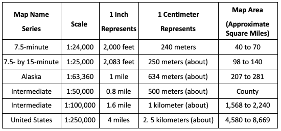
A convenient way of representing map distance is by the use of a graphic scale bar. Most topographic maps have scale bars in the map margin that represent distances on the map in miles and kilometers. Accuracy of horizontal distances is better than 1/50 inch on maps of scale 1:20,000 or larger, and 1/30 inch on maps of smaller scale. Therefore a map of 1:24,000 (larger scale) has a horizontal accuracy of 40 feet.

Large Scale versus Small Scale – Large-scale maps show features larger on the map than a small-scale map. A feature shown on a map of scale 1:24,000 will be drawn in a physically larger size on that map than the same feature drawn on a map of scale 1:100,000. Therefore the map of 1:24,000 scale is said to be a “larger scale ” map compared to the 1:100,000-scale map and the 1:100,000-scale map is said to be a “smaller scale” map compared to the 1:24,000 scale map. More detail can be seen on a “large-scale” map, but more territory (with less detail) can be shown on a small-scale map. Large-scale maps are generally better for more precise land navigation and terrain assessment, however smaller scale maps can give a better perspective of the entire area, which is useful when planning search strategy.

Topographic Contour – A topographic contour is a line drawn on the map to represent a terrain path of constant elevation. Topographic contours are drawn as a series of continuous roughly parallel lines (in the sense that they do not intersect), with spacing between the lines that represents a fixed change in altitude. Typical contour intervals may be 20, 40, 50, or 100 feet, depending on the map, but is fixed for any given map. If a person walking on a hill could follow a contour line, they would follow a path of constant elevation, not going uphill or downhill. If one traveled perpendicular to the topographic contours one would be traveling straight uphill or straight downhill.

Topographic contour lines come as “Index” lines, “Intermediate” lines, and “Supplementary” lines. Index lines, which are darker thicker lines, are labeled with a number representing elevation. Typically every fourth or fifth line is an index line. If the index lines were every fifth line and the contour interval was 20 feet, the elevation change between successive index contours would represent 100 foot of elevation change. In this case the Index lines would be drawn at elevations, which are exact multiples of 100 feet. Intermediate contour lines lie between Index lines with a spacing representing the contour interval, but they are not labeled. Supplementary contour lines resemble dashes. They show changes in elevation of at least one half the contour interval and are normally found where there is very little change in elevation, such as on fairly level terrain. 40-foot contour intervals are the default for SARTopo, although others may be used. In that case, index contours drawn as every fifth line represent multiples of 200 feet elevation change. Elevation accuracy is better than one-half the contour interval.

Contour Interval – The change in terrain elevation represented on a map by the spacing between intermediate topographic contour lines.

Datum – The datum is the reference shape of the Earth on which coordinates are laid for drawing map features and determining position. This is only important when comparing coordinate information between two different map sources. If the maps do not use the same Datum, then the coordinates may be slightly off. The North American Datum 1927 (NAD 27) is used on most local USGS Quad maps. The World Geodetic Survey 1984 (WGS 84) is used for most military maps and is the default Datum used in GPS receivers, although GPS receivers allow selection of Datum (see section below on GPS). The difference between NAD 27 and NAD 83 (new DATUM used by the USGS) is represented by dashed corner tics on the map (look closely). The difference between NAD 83 and WGS 84 is negligible, so the dashed corner tics also effectively represent the difference between NAD 27 and WGS 84. This difference is 47 meters (1.9 seconds of longitude) or less East-West and 1.5 meter (.05 seconds of latitude) or less North-South, in El Paso County. Within Colorado, the difference can be as great as 59 meters East-West and 4.5 meters North South. EPCSAR standard datum is WGS 84.

Maps Used by EPCSAR
Several different types of maps are used by EPCSAR personnel.

SARTopo Maps
Maps printed from the online tool https://sartopo.com/ replaced USGS maps in 2022 as the EPCSAR standard. SARTopo data is updated several times a year from various sources including https://www.openstreetmap.org/ The mapping software not only allows us to print up-to-date maps for field use but also enables teams with mobile devices to send and receive information. This real-time communication allows search planners to track field teams and provide feedback to their destinations.

USGS Maps
Although EPCSAR no longer uses USGS maps, our sister teams in the state still do. Therefore they remain relevant for mutual aid and out-of-county missions.

The United States Geological Survey has systematically divided the United States into a series of precise quadrangles. There are several series of these maps, each using quadrangles of a different size.

The most useful are maps from the USGS Primary Map Series, which uses a 7 ½ minute quadrangle (7 ½ x 7 ½ minutes) at a scale of 1:24,00. It takes 1,881 of these maps to cover all of Colorado. These are the largest scale maps available, i.e., they show more detail, and in that respect are one of the best for wilderness navigation. The section below on Map Reading focuses on this series of map.

Other USGS quadrangle series include Quadrangles covering 30 x 40 minutes at a scale of 1:100,000, taking 56 quadrangles (maps) to cover Colorado; and Quadrangles covering 1 x 2 degrees at a scale of 1:250,000, taking 16 to cover Colorado. The USGS also publishes a series of County Maps with scales of 1:100,000 and 1:50,000, which show selected natural and cultural features. Four of these County Maps cover El Paso County. County maps are not available for all areas.

Pikes Peak Atlas
The Ormes’ Pikes Peak Atlas is a large folded, double-sided map that is a standard within EPCSAR. Every member should carry a copy. It uses a smaller scale than the USGS 7/1/2 minute Quads, namely 1:36,000 and a contour interval of 100 feet, but covers considerably more area. It’s main value is that is covers all mountain areas within El Paso County, it is one of the best labeled maps for trails, forest service roads and names of various geographic features. L and longitude are indicated in the margins and it is printed on waterproof paper. It is a good backup for when you travel off the edge of the Quad you may be carrying.

El Paso County Map
This map does not have topographic features, but has value for showing roads in the eastern part of the county.

Trails Illustrated Series Maps
The Trails Illustrated Map #137, “Pikes Peak/Canyon City” is good because it covers a large area surrounding Pikes Peak, it is a topographic map with a contour interval of 80 feet and scale of 1:66,667, it labels most trails and Forest Service roads, and it is printed on tear-proof, water-proof material. It is another good backup for when you find yourself traveling off the edge of the local Quad you carry. It is also good when supporting missions in Teller County.

Forest Service Maps
Forest Service Maps provide coverage of National Forest Areas. They are good for showing forest service roads and accurate demarcation of public and private property lines.

The MacVan Map of Colorado Springs, Pikes Peak Region and Pueblo, Street Guide
This is a book map of Colorado Spring and surrounding areas. It is one of the best, most detailed, and up to date street maps of the local area. All members are strongly encouraged to have a copy. Mission pages requiring staging in residential or rural areas will frequently cite the page number in the book and map reference grid to help members locate the EPCSAR staging area for the mission.

EPCSAR Maps

Maps in EPCSAR Rescue Vehicles
There is a packet of maps in all primary rescue vehicles. The packet includes the Pikes Peak Atlas; copies of several local Quads; a county map; and The MacVan Map of Colorado Springs, Pikes Peak Region and Pueblo, Street Guide. These may be used while with the vehicle, but are not to be removed and taken into the field unless told to do so by the Incident Commander.

Map Reading
The primary maps used by SAR teams in the field are printed from https://sartopo.com/. The discussion on map reading will focus on use of these maps.

Information on the Map Margin
This section will point out some of the key information found in the margins of SARTopo maps. A more complete description of information found in the margin can be found in reference 5.

The zone of the map appears in the lower left-hand corner along with the map datum. It is useful to note the “Datum” if one is using a GPS receiver or comparing information between two different maps

The map scale appears in the center of the lower margin. The scale is given as a ratio and as a set of linear measurement scales in miles and kilometers. Distances on the map can be measured by marking the edge of a piece of paper to show the distance scale then use the paper to measure distance on the map. Alternatively, one can mark the separation distance between two points on the edge of a piece of paper, then compare the paper marks to one of the distance scales. If one has a ruler, or has a ruler marked on the edge of one’s compass, it is useful to remember that with a scale of 1:10,000, one centimeter equals 100 meters.

Some compasses have plastic base plates with markings for several different map scales.

Magnetic North and Magnetic Declination are shown in the lower right-hand margin. These are discussed further in the section on the use of a Compass.

The UTM coordinate systems is also marked along the edges of the map. This will be covered in a later section.

Map Symbols
Symbols on the map represent various types of natural and man-made features. Symbols are color-coded as follows:

• Red and black represent man-made features

• Brown is used for topographic features using topographic contours

• Green represents vegetation

• Blue represents water

Note that grey shading is used to depict features such as buildings, water tanks, and wells. Trails are red. Other roads, railroads, boundaries are shown in black.

The transition between vegetation areas in green and barren areas or clearings in white can provide a useful reference when navigating by terrain.

Interpreting Topographic contours

Topographic contours are by far the best tool for assessing terrain and locating oneself on the map using terrain features. Topographic contours can help an individual gain a 3-dimensional visualization of the terrain. Hills, gullies, peaks, and valleys are easily identified. The following provides some examples for interpreting topographic features.

Slope:

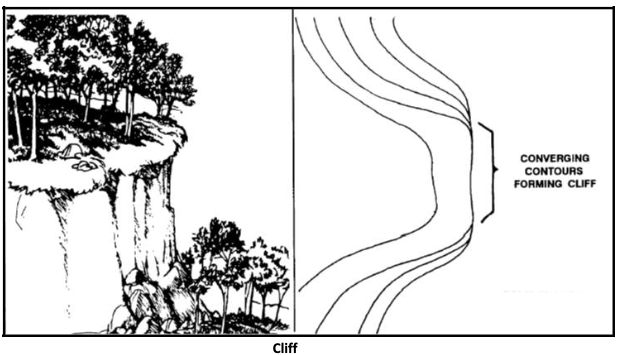
You are going uphill if you cross contour intervals of greater elevation and you are going downhill if you are crossing contour intervals of decreasing elevation. The steeper the slope the closer the contour lines. Lines so close they touch or merge to one line, represent a cliff. Wide-spaced lines represent relatively flat areas. Keep in mind the contour interval and scale when judging slope. A larger contour interval will tend to show a wider spacing for the same slope and a smaller scale will tend show closer contour lines for the same slope. Note that given map scale and contour interval, some relatively small features may not be possible to show on the map. A small cliff, making a route impassable, may not show on the map.

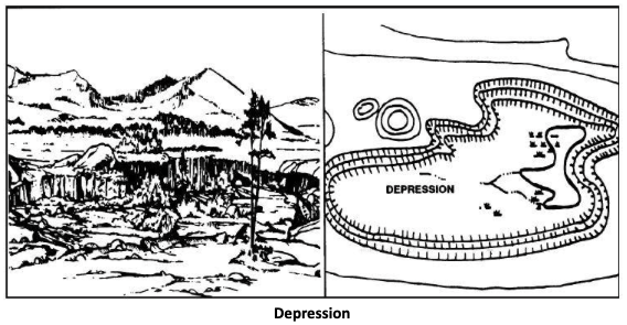
Peaks and Depressions:

The area near peaks of mountains and hilltops or near a depression appear as local concentric contours as shown in the figure:

 Contour Lines Showing a Hill or Depression

The distinction of whether this is a hill or depression depends on whether contour lines at the center show increased or decreased elevation compared to the outer contour lines. In areas where there is uncertainty of whether the contour lines are showing a hill or depression, mapmakers add hash marks to the contour lines, which always point downhill. A peak may have an “x” in the middle with the elevation indicated to show the exact location of the summit.

A Pass or Saddle:

A pass or saddle has higher elevations on two sides and lower elevations on the other two sides, yielding a characteristic hourglass shape.

 Contour Lines Showing a Pass or Saddle

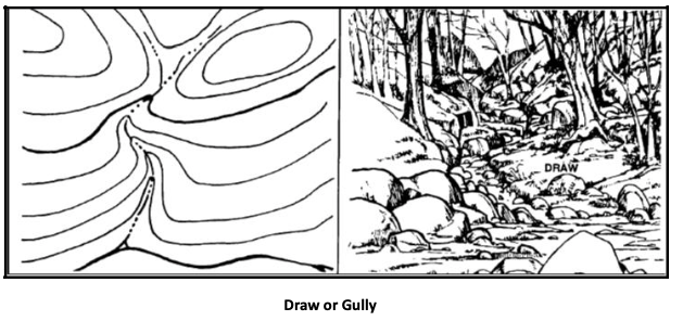
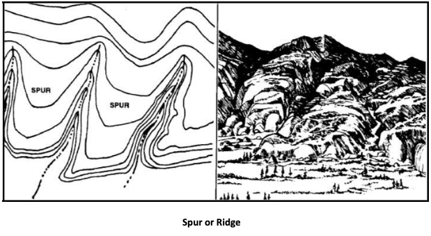
Ridges and Valleys (ravines and gullies):

Ridges and valleys show as a series of U’s or V’s pointing in the same direction as shown in the figure.

Contour Lines Showing Ridges and Gullies

Generally ridges show as more U-shaped (rounded) contours and gullies or ravines show as more sharply shaped V’s (sharper), but this is not always the case. The distinction shows with the direction of decreasing or increasing elevation. Gullies have contours, V’s or U’s pointing uphill and ridges have contours pointing downhill. Also, if there is a stream (thin blue line) indicated in the center of the V’s or U’s, it is a gully, but if the steam is on the edge of the V’s or U’s, it is a ridge.

Terrain Comparison:

U.S. Army Field Manual FM 21-26 (Reference 3) has some good figures comparing topographic contours with terrain. Some of these figures are reproduced below:

COMPASS

Compass Directions
Remember that angle measurements in degrees are defined by dividing a circle into 360 parts. A compass face is simply a circle marked off in degrees from 0 to 360. Compass readings are referred to as “bearings”. Compass bearings are measured clockwise from North with the four points of the compass (North, East, South, West) shown at 90-degree intervals, that is intervals of ¼ of the circle. Starting with North at 0 (or 360) degrees, East is at 90 degrees, South is at 180 degrees, and West as is at 270 degrees.

Compass Errors
Compass needles are small bar-magnets that work by aligning with the local direction of the Earth’s magnetic field. Because they are magnets they can be drawn off by interfering magnetic fields originating from metallic objects (principally iron and steel) or magnetic fields created by electronic devices. Usually the cause is manmade: knife, belt buckle, eyeglass rims, camera, binoculars, zipper, wire fence, power line, ice axe, or radio. If it’s close enough to the compass, even an object as small as a paper clip can cause drastic errors. It is important when taking compass readings, to make sure there are no metallic or electronic devices nearby.

Also, a bubble can form in the liquid within the housing of a compass with changing air pressure, especially in severe cold. A bubble larger than 1/4 of an inch can nudge a needle and produce a false reading.

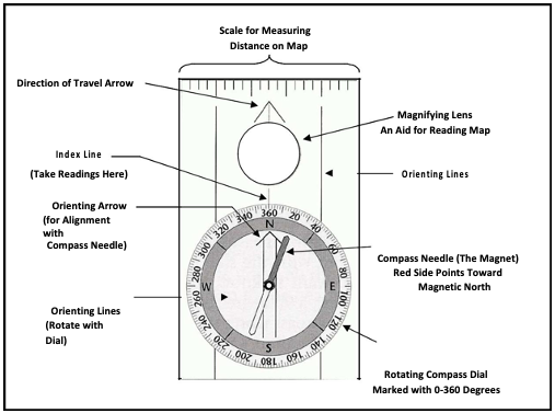
Using a Compass
First remember these rules for maximum accuracy:

• Hold the compass directly in front of you.

• To align the magnetic needle and the orienting arrow, hold the compass close enough so that you look down in the face, not at an angle.

Each degree of error in measuring an angle amounts to about 92 feet error in position at 1 mile.

You need to know the following basic compass skills:

Set a Bearing

Use this technique when you want to travel on a given bearing using your compass to determine the correct direction.

• Turn the compass dial until the desired bearing is aligned with the index line.

• Turn your body and the compass until the north-seeking end of the needle (Red End) is aligned with the pointed end of the orienting arrow.

• The direction-of-travel arrow now tells you which way to travel to follow the desired bearing.

Measuring a Bearing

Measuring the bearing from your position to some landmark can help you determine your position or can be an aid in communicating your position. This is done simply by reversing the steps for setting a bearing.

• Point the compass’s direction-of-travel arrow at the landmark.

• Turn the compass dial until the pointed end of the orienting arrow aligns directly under the north-seeking end of the compass needle.

• Ensure that the direction-of-travel arrow is still pointed at the landmark.

• Read the bearing at the index line.

Following a Bearing

The trick to staying on a given bearing is to pick intermediate landmarks along the line from your location to your destination, traveling the distance in short legs. Follow these steps:

• After determining the bearing to your destination, set the bearing on your compass. (Determining a bearing from a map is covered later.)

• Look ahead along the direction-of-travel arrow and select an intermediate landmark you can keep in sight and walk to from your starting point.

• Now ignore the compass and walk to the landmark by the easiest route, but do not change the setting on the compass dial!

• When you reach the landmark, take out your compass, verify that the correct bearing is still set on the index line, and by rotating yourself and the compass, align the north-pointing end of the compass needle with pointed end of the orienting arrow. Don’t turn the compass dial!

• Select another intermediate landmark along the bearing line and walk to it. Repeat this process as often as necessary until you get to your destination.

• If you cannot find a convenient landmark, perhaps due to fog, simply use your partner as a portable intermediate landmark.

Keeping on Your Bearing by Backsighting

When traveling along a line of sight between landmarks, you may occasionally lose sight of the landmark or become confused as to the identity of the landmark you were headed for. Your landmark boulder may look very similar to another forty feet away. To check:

• Sight back to the landmark you just came from.

• Point the direction of travel arrow at it. Don’t turn the compass dial!

• If you are on the correct line of travel the south end of the needle will be aligned with the pointed end of the orienting arrow. If it isn’t, simply move right or left until it is.

• Face your intended direction of travel and reacquire your next landmark or acquire a new landmark if the other still cannot be distinguished.

Backbearings

Once you have reached your goal, it may be necessary to return to your starting point. The simplest way to do this is to follow a back bearing. There are two ways to follow a back bearing.

• Determine the new return bearing

• Reset it on your compass following the steps above, traveling by intermediate landmarks

Alternate method

• Don’t change the compass heading you arrived on (this eliminates the possibility of mathematical error).

• Turn the compass until the south end of the needle lines up with the pointed end of the orienting arrow. (Just the same as in backsighting.)

• Travel back to your starting point using intermediate landmarks.

Travel to a Baseline

This is one of the simplest applications of compass skills. A baseline is a long fairly linear landmark whose direction from your location is known, and that when reached, will guide you to your desired destination.

Often areas will include power lines, a ridge, a road, or a river. When choosing a baseline, make sure that it is a permanent and readily identifiable feature. Streams can dry up in the summer. Trails that are easily recognized in summer can disappear when snow covered. What is important is that you know the direction to the baseline from your location, so that you can hike to it, then to where you want to go along the baseline.

Say that there is a north south ridge to the west of you and a road out that crosses the ridge about two miles south. Simply set your compass for a bearing of 270 degrees and when you reach the ridge, follow the ridge south until you reach the road, then follow the road.

Deliberate Error

Sometimes when traveling to a location on a road or trail, it may be useful to introduce an error to one side or the other of your destination to ensure an efficient arrival. This is especially useful if you are not sure of the exact location of what you are looking for along the trail or road.

Say you are hiking west after leaving your car on a north-south section of the Mt. Herman Road. If you try to return to your car by using an exact bearing chances are that you will miss it. Even worse you may not know whether you reached the road north or south of your car. Deliberate error makes the right guess for you. Instead of following a direct bearing, follow a bearing that will deliberately plan to reach the road to one side or the other. Plan a large enough deliberate error to account for any uncertainty in your cars location. Then when you reach the road you will know which way to turn. If you have one mile to go, introducing a deliberate offset of 10 degrees in the bearing will provide you an offset of just under 1000 feet along the road from your car. A smaller deliberate error can be used when traveling a greater distance. Deliberate error is useful in any situation where you want to reach a point on a line, e.g., a bridge over a river, a pond on a stream, your camp at the base of a ridge.

Getting Around Obstacles

Assume you have taken a bearing to your goal and are proceeding to it using intermediate landmarks when you come over a rise and find that some one has damned the small creek shown on the map and now there is a sizable pond right on your direction of travel. There are two solutions to this problem both of which will put you back on the right course.

First solution:

• Note the point at which you are going to deviate from your desired direction of travel. Mark your location with something such as a pile of rocks,

• Sight to the opposite shore and select a landmark on your bearing line. Make your way to the landmark on the opposite shore

• Backsight to the point at which you left your direction of travel. (This will eliminate any doubt that you are back on the correct course.)

Second solution:

In the case when you can’t see past the obstacle another method must be employed. It involves pacing away from the course at a known angle -preferably a right angle-

• Before you begin to maneuver around the obstacle, turn around and backsight along your travel line into the distance. There may be some feature tall enough to be seen from beyond the obstacle, once you clear it and move away from it. Now facing the obstacle along your bearing turn at a right-angle (90º) [right or left whichever direction provides the best route around the obstacle] and walk until you are past the obstacle, counting your steps as you go. (Write down the number.)

• Once past the end of the obstacle, resume your original bearing and move forward again until you are past the obstacle.

• Make a right-angle turn heading back to your original course and go the same number of steps.

• If the obstacle is very large you can measure the distance in elapsed time rather than steps. The compass faceplate lets you make the right angle turns without doing any calculations or resetting bearings. This eliminates the possibility of mathematical errors and forgetting your original bearing. Simply sight along the back edge of the base plate.

Tips for the Real World

• Make careful, accurate sightings for both destinations and intermediate landmarks.

• Follow the direction-of-travel arrow not the compass needle when walking a bearing. (The compass needle must be aligned in the orienting arrow when following the direction-of-travel arrow.)

• To avoid an accumulation of small errors, recheck bearings carefully and use bearings over short distances whenever possible.

• Aim for a line rather than a point, when feasible. For instance a stream is easier to hit than a bridge over the stream.

• Line up two distant objects on your bearing-line that will always be in sight.

Continually relate your progress to the map.

Magnetic Declination
A magnetic compass needle aligns with local magnetic field lines and does not point to true North. The deviation of the compass needle from true North is called “Magnetic Declination”. The direction a magnetic compass needle points is called “Magnetic North”. A bearing referenced relative to Magnetic North is referred to as a “Magnetic Bearing” and a bearing referenced relative to True North is referred to as a “True Bearing”. When relating compass measurements to a map one must compensate for magnetic declination. When reporting bearing one should always state whether one is referring to a magnetic or a true bearing. All EPCSAR members must be able to convert between magnetic bearing and true bearing.

The magnetic declination in our location (Colorado Springs) is about 8 degrees east of True North. That is, the north-seeking end of a compass needle will point to a direction 8 degrees to the east of True North.

A USGS web site (http://www.ngdc.noaa.gov/geomag/) provides the means for calculating magnetic declinational at any given location:

Using the USGS web calculator for Colorado Springs (38 52’ 30” N / 104 52’ 30” W and altitude of 6,400 feet, i.e., the SE corner of the Cascade Quad, for 19 September 2016) one gets a magnetic declination of 8.35 degrees East and a rate of change of –6 minutes per year (-.100 deg/year). [Using the World Magnetic Model 2015, expiring in 2019.] Given that rate of change, one does not have to worry about changing one’s magnetic declination setting from 8.5 degrees East to for at least another 2 years (from Sep 2016).

Converting Between Magnetic and True Bearings

The figure below relates Magnetic Bearings to True Bearings. Note that with Magnetic North to the East of True North, as in Colorado, one can convert between Magnetic and True North as follows:

True Bearing = Magnetic Bearing + Magnetic Declination

and

Magnetic Bearing = True Bearing – Magnetic Declination

Maps are always oriented to True North (left and right borders are aligned North-South). Magnetic compass needles always point to Magnetic North. Therefore if one relates a field compass measurement to a map, and vice versa, one must convert from a magnetic bearing to a true bearing and vice versa. Some individuals like to remember the conversions by the phrases: Field to Map Add (FMA) and Map to Field Subtract (MFS).

Some compasses have adjustments for magnetic declination. Once set for the appropriate magnetic declination, one reads True Bearings when making compass measurements.

If you don’t know the magnetic declination at your location, you can determine the declination by standing at a known point marked on the map and taking a magnetic bearing to another known point on the map. Then measure the true bearing on the map. The declination is given by subtracting the magnetic bearing from the true bearing. A positive value gives a declination to the east of true north and a negative value gives a declination to the west of true north.

                                                  Relating True and Magnetic Bearings

Map and Compass Together

Orienting a Map:

Orienting a map means rotating your map so that the top and bottom of the map are oriented towards True North and True South respectively. When your map is oriented, then real world features lie in same direction as they do on the map. That means that a line drawn on the map from your location to any landmark will actually point toward the real world landmark. When you do this, you can better relate terrain features around you to the map and determine a more accurate estimate of your position or better assess the direction you must take.

If Your Compass Has Been Adjusted To Compensate For Magnetic Declination:

• Align north on the compass dial with the index line.

• Set the compass on the map and align the edge of the compass with the edge of the map (north toward the top of the map).

• Rotate the entire map together with the compass until the north-seeking end of the compass needle (Red End) is aligned with the pointed end of the orienting arrow. Your map is now oriented

If Your Compass Has No Compensation For Magnetic Declination:

• Align the compass dial so that 351.5 degrees aligns with the index line. (True north is 8.5 degrees to the west of magnetic north in Colorado.)

 Follow the last two steps in the preceding case.

Taking A Compass Bearing From A Map:

When doing the following steps, ignore the compass needle and all markings inside the compass dial. You are using your compass only as a protractor to measure angles.

• Draw a straight line on the map passing through your location and running through your destination and extend the line across any one of the map borders

• Center the compass where the line you drew intersects the map border and align the direction-of-travel arrow along the line. (See Figure 13-10)

• Turn the compass Dial so that N-S or E-W aligns with the map border, and read the true bearing on compass circle at the index line. Be careful to get the bearing in the correct sense because a straight line will have two values 180° apart. Remember north is 0, east is 90, and so on.

If you then want to convert this to a magnetic bearing, subtract 10 degrees (the magnetic declination). The procedure is exactly the same to determine the bearing between any two points on the map.

        Determining a Bearing from a Map

Plotting a Compass Bearing on a Map

Let’s say you want to triangulate your position on the map. From your location, you take bearings to two different landmarks. For best accuracy, the two landmarks should be close to 90 degrees apart.

Do this separately for each landmark. Ignore the direction of the compass needle in all these steps:

• Locate a landmark on the map that you can actually see from your location.

• Take a compass bearing to the landmark. If your compass is not compensated for declination, then add 8.5 degrees to the measured magnetic bearing (you want to plot a true bearing on the map).

• Turn your compass dial so that the true bearing is aligned with the index mark.

• Carefully fold one side of the map so that the edge of the map passes close (within a half compass width) to the landmark, but do not cover the landmark. Keep top and bottom edges of the map exactly aligned so that the folded edge will be oriented North-South.

• Set your compass on the map and align an edge of the base plate with the edge of the map and draw a North-South line next to the landmark, then unfold the map.

• Holding the compass with North on the compass dial towards the top of the map, place the compass on the map with one edge of the base plate on the landmark. Then keeping the edge on the landmark, carefully rotate the compass base plate (do not rotate the dial) so that one of the orienting lines inside the compass dial aligns exactly with the North-South line you drew on the map.

• Draw a line along the edge of the base plate that touches the landmark.

• Since you are triangulating from the landmark, extend the line along the back bearing. If you were plotting a bearing from a landmark, then you would extend the line along the bearing.

When this is complete for both landmarks, extend the lines to see where they intersect. Your location is the point of intersection. You can check accuracy by plotting the bearing to a third landmark.

Land Navigation Using Map and Compass

Determining Position

Terrain association: Using terrain association means relating features on your map to your real-world surroundings. Terrain association is done by visualizing the three dimensional terrain using terrain contours, and by using demarcations such as vegetation areas, clearing, and other natural or man made features (e.g., creeks or rivers, trails, trail intersections, power lines, or roads – basically anything represented by a symbol on the map) as reference points to the real-world. Terrain association using contour features is best done continuously as one moves. If one moves without a continuous conscious awareness of how one is following the terrain, it may be difficult from terrain association alone to determine which ridge or gully one is following. It may require one’s taking bearing measurements to known features, or reaching a specific map feature in order to eliminate the ambiguity. Ridges and gullies have a habit of branching off as one goes down hill. You must be aware of where you are at each decision point. Following the wrong ridgeline or gully is a major cause for people getting lost. This is something to consider when planning a search. Also, some ridges and gullies may be too low or shallow to show up well on the topographic map. Be aware of the ridge heights and shallowness of gullies relative to the contour interval of the map.

An altimeter is very useful resource to determine ones position. If one is on a trail, known ridgeline, or gully, an altitude measurement may be sufficient to provide one’s precise location.

Triangulating: Triangulating ones position involves plotting compass bearing from landmarks as described in the previous section. The intersection of the bearing lines is your position. If you are following a trail or other linear feature (ridgeline, gully, power line, etc.), one bearing measurement is enough to determine your position along that feature. Beware of false summits when using peaks for bearing measurements.

Determining Best Route

Determining the best route involves assessing the terrain and avoiding obstacles. This may be necessary when navigating to a given destination or for estimating a lost subject’s likely route. One factor in assessing terrain is the slope, whether uphill, downhill, and steep or flat. Steepness can be determined by the spacing of contour lines. Compare the terrain at your location to the spacing of contour lines on the map at your location to get a perspective for the slope at other points on the map. Plan a route that avoids unnecessary changes in altitude, i.e., avoid too many ups and downs if possible. You want as direct a route as possible that is safe. Due to the scale and contour interval of the map, you cannot expect to identify all obstacles. There is no substitute for experience, query your team members to see if someone is familiar with alternative routes.

MAP COORDINATES

Coordinates divide maps into small units that allow any specific location on the map to be referenced by citing the coordinates of that location. Coordinates are therefore a convenient means for locating oneself on a map and for reporting one’s position precisely. The Township/Section coordinate system has already been discussed. This section will focus on Latitude/Longitude and the Universal Transverse Mercator (UTM) coordinate systems. EPCSAR members should be familiar with both. SARTopo maps are labeled with the UTM coordinate system, but the Ormes’ Pikes Peak Atlas and Trails Illustrated maps only reference Latitude/Longitude.

Geographic Coordinate Grid (Latitude/Longitude)

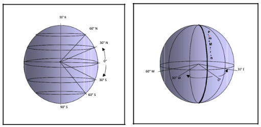
The system known as the geographic coordinate system uses lines of latitude and longitude to locate points on the surface of the Earth. Lines of latitude are circles around the globe going east and west that are parallel to the equator. The lines of latitude are referred to as “parallels of latitude” or just “parallels”. Lines of longitude a re circles that run north and south around the globe, all intersecting at the north and south poles, and are perpendicular to parallels of latitude. A longitude line running from pole to pole (half circle) is referred to as a “meridian”.

                                       Lines of Latitude (Parallels) and Longitude (Meridians)

The distance of a point north or south of the equator is known as its latitude. The measure of latitude (how far north or south) uses divisions of a circle in degrees as shown below. Latitude runs from 90º north to 90º south.

                                Measuring Latitude               Measuring Longitude

Longitude is also measured in degrees. The angle is measured in the plane of the equator based on where a given meridian intersects the equator. (See figure above) One meridian is designated as the prime meridian and all angles are measured east or west from the prime meridian. The prime meridian of the system we use runs through Greenwich, England and is known as the Greenwich meridian. The distance east or west of the prime meridian to a point is known as its longitude, and can range between 180º east and 180º west. The meridian at 180º east is the same as the meridian at 180º west and is known as the International Date Line. The International Date Line is part of the same circle as the prime meridian, but is the half on the opposite side of the earth.

When specifying latitude or longitude to a precision finer than one degree, one can use “minutes” and “seconds” there being 60 minutes in one degree and 60 seconds in one minute. One can also use fractional degrees instead of minutes and seconds or fractional minutes instead of seconds. Degrees, minutes and seconds are indicated by the symbols: º, ‘ , and ” respectively. Thus a latitude of 38 degrees, 45 minutes, and 30 seconds north, would be represented as: 38º 45’ 30” N. Given that 30” is half of one minute (30/60) or .008 degrees (.5/60) and that 45’ is ¾ of one degree, that latitude could also be represented as 38º 45.5’ N or as 38.758º N.

At any point on the earth, the ground distance covered by one degree of latitude is about 111 kilometers or about 69 statue miles, or exactly 60 nautical miles (one nautical mile was originally defined as the distance corresponding to one minute of latitude or one minute of longitude at the equator). One second of latitude is equal to about 30 meters or 100 feet.

The ground distance covered by one degree of longitude at the equator is also about 111 kilometers, but decreases as one moves north or south, because meridians converge at the poles. One second of longitude represents about 30 meters or 100 feet at the equator; but at the latitude of Colorado Springs (38º 50’ N), one second of longitude is approximately 24 meters or 79 feet.

The four lines that enclose the body of a USGS quad map (neatlines) are latitude and longitude lines. Therefore the neatlines on each side of the quad run exactly north-south and the neatlines at the top and bottom of the map run exactly east-west, and their coordinate values are given in degrees, minutes, and seconds at each of the four corners. 

USGS quads of scale 1:24,000 in our area, show 7 ½ minutes of latitude by 7 ½ minutes of longitude. Tic marks on each edge of the map extending in from the border (neatlines) are labeled at units of 2 ½ minutes (2’ 30”) of latitude and longitude. These latitude/longitude tic marks divide each edge of the map into thirds (since 3 times 2 ½ minutes equals 7 ½ minutes). If one extended these tic marks across the map, one would note that there is a cross (“+”) at interior points in the map where north-south and east-west tic-lines would intersect. This is represented in the figure below, as it would show on a USGS 7 ½ minute quad (actual values shown in the figure are for the Cascade quad).

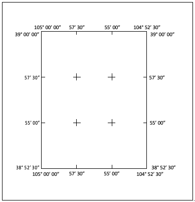
              Latitude and Longitude Markings on a

Representative USGS 7 ½’ Quad Map

The geographic coordinates of a point are found by dividing the sides of the geographic square in which the point is located, into the required number of equal parts. Given tic marks on each side denoting an interval of 2’ 30”, which is equal to 1 50” (60” + 60” + 30” = 2 ½’), one needs to divide the interval into 150 equal parts, each corresponding to one second of latitude or longitude. This could be done with a metric ruler 30 centimeters (300 millimeters) in length, where every two millimeters represents one second of latitude or longitude. [A 15-centimeter ruler would be too short since it would not reach between the tic marks on a 7 ½ minute quad.]

To use the ruler, one needs to either draw lines between the tics bounding the location on the map one wishes to measure, or fold the map to align with the tics. The ruler should then be laid on a slant between the lines so that the 0 and 30 cm marks on the ruler align with the tic-lines as shown in figure 13-15. Even though the ruler is on a slant, it still divides the space between the two tic-lines into 300 equal divisions. If one measures the point of interest on the map at 226 mm, that is 113”, above the 55’ 00” tic line, then the latitude of the point is 38º 56’ 53” N. This is computed by noting that 113” equals 60” + 53”, which equals 1’ 53”, which must be added to 38º 55’ 00”, giving the result. If one did not have a ruler, one would have to make a rough judgment, for example looking at the figure, that the point of interest lies ¾ of the distance between the two tic-lines. ¾ of 150” equals 113” when rounded to the nearest second, which coincidentally in this case (a lucky judgment call), gives the identical latitude as when measured using the ruler. The same technique can be used to measure longitude.

Use Of 30 Cm Ruler To Read Coordinates Between The Lines.

Universal Transverse Mercator (UTM) Grid

UTM stands for Universal Transverse Mercator, a type of projection used to produce a flat map. A Mercator projection, projects the surface of the Earth onto a cylinder whose axis coincides with the Earth’s North-South axis and that is tangent at the Equator. Gerardus Mercator first used the cylindrical projection in 1569. A transverse Mercator projection uses a cylinder rotated by 90 degrees (transverse cylinder) so the cylinder is tangent at one meridian. 

Transverse Mercator Projection

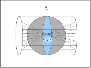
To limit distortion, so that distances are uniformly scaled in all directions and so that angles are represented correctly on a flat map, the projection for each cylinder is limited to a sector 6 degrees wide and only runs from 80º south latitude to 84º north latitude. To cover the poles, the UTM grid system is used together with the Universal Polar Stereographic (UPS) grid. The UPS grid system doesn’t concern us here in Colorado, but you may encounter it when for example, selecting a coordinate system to use in a GPS receiver, which may be represented as “UTM/UPS”.

The UTM grid system divides the Earth between latitudes 80º south and 84º north into 60 sectors as shown in figure 13-16, each 6º wide (6º of longitude). Each sector is then divided into zones representing either 8º or 12º of latitude. (Only the zones between 72º and 84º north latitude use zones 12º high. 

When projected on the cylinder and opened out flat, The UTM grid system looks as shown in Figure 13-17. Sectors (columns) are counted from 1 to 60 starting at 180º west longitude going east. East-West bands are labeled alphabetically from south to north with the poles using A,B (South Pole) and Y,Z (North Pole) in the UPS grid system. Also, the letters “I” and “O” are not used. The UTM grid system produces a system of horizontal and vertical perpendicular grid lines. UTM grid references are always given going east, referred to as “Easting”, and then going north, referred to as “Northing”.

 UTM Zone Structure Showing Location of Colorado

                                              UTM Zone Structure Showing Location of Colorado

The majority of Colorado lies in UTM Zone 13S, as shown in the figure. The western part of Colorado from Delta Colorado west, is in sector 12 and the northern part of Colorado from Boulder north, is in band “T”.

The unit of measure in the UTM grid system is the kilometer. Each Zone is covered by a set of 100 Km squares, each of which is subdivided into 10-kilometer squares, which again are divided into 1-kilometer squares. The 1-kilometer squares are represented by blue tic marks on each side of USGS quads. The 1-kilometer squares can then be divided into 100-meter units, then 10-meter units, etc. to get as precise a coordinate specification as desired.

To avoid having to specify east-west or using positive and negative numbers, the UTM system uses a separate false origin for each Zone. The origin for east-west measurements is set at the center of the zone and is arbitrarily set at 500,000 meters (500 kilometers). The north-south origin is set to be zero at the equator. Therefore Northing units represent the position in meters, north of the equator, whereas Easting units are given in meters with 500,000 meters representing the center meridian of the Zone. Given that the largest east-west size of a 6º-wide Zone is 668 kilometers (a Zone on the equator), an Easting coordinate always falls between 166000 E and 834000 E (that is 500,000 ± 668,000/2). In Colorado, Easting coordinates always fall between 233000 E and 767000 E and Northing coordinates are always greater than 4090000 N and always less than 4550000 N (i.e., the southern border of Colorado is more than 4,090,000 kilometers north of the equator).

USGS quads have the UTM grid referenced as blue tic marks along the border, showing the demarcation of each 1-kilometer UTM grid square. (See Figure 13-18.) The UTM Zone (e.g.

“zone 13”) is given in the text on the left side of the map in the bottom margin. Usually, one tic mark on each side of a USGS quad is labeled down to the meter, e.g., ⁵10^000mE or ⁴³03^000mN,

whereas other tic marks drop the three zeros at the end and therefore represents coordinates in kilometers (e.g., ⁵09 and ⁴³04). The superscript portion at the start of each coordinate represents the 100-kilometer grid reference. A complete UTM coordinate specification would be given stating the Zone and then giving the Easting coordinate followed by the Northing coordinate, e.g.,

13S 0510921E 4303455N

In this example, coordinates are given down to the meter, meaning the position has been measured or estimated inside the 1-kilometer grid square.

In most practical circumstances, there is no need to give the Zone reference and there will likely be no confusion between Easting and Northing coordinates, because they differ significantly. This then is one of the useful practical sides of using the UTM grid. If one is given coordinates in any order, even without specifying N or S, one can match up the coordinates with those given in the margin and quickly determine which is which.

               SE Corner of Cascade Quad Showing UTM Coordinate Markings

The best way to read UTM coordinates off a map is to draw the UTM coordinate lines connecting the tics on opposite sides of the map and then either estimate the decimal fraction of distance between the lines for the point of interest on the map; or use a 10 cm ruler in a manner similar to the manner described for reading latitude and longitude; or purchase a plastic template that divides the 1 kilometer square into 100 meter squares. One can also fold the map instead of drawing lines on the map, but the map edge running across the map must align with the tics on opposite sides of the map. This can be accomplished fairly easily by aligning to one tic and folding the map so that the overlapping edges align with each other. This works because as discussed in the next paragraph, for all practical purposed the UTM N-S grid gridlines can be taken as True North and the up-down edges of the map also align to True North.

The deviation of UTM vertical lines from North is shown in the bottom margin of the map where True North and Magnetic North are shown. The line labeled “GN” shows the orientation of UTM vertical lines relative to True North and Magnetic North (MN). In our area, UTM vertical lines are either 2 minutes (1/30 degree) east of True North or 2 minutes west of true north depending on the map (e.g., 2 minutes west of True North on Woodland Park quad and 2 minutes east of True north on Cascade quad). This difference is insignificant for SAR field-work (e.g., 1/30 degree equates to a distance error of less than 6 meters at 10 kilometers).

GLOBAL POSITIONING SYSTEM (GPS)

The GPS System uses a constellation of 24 satellites in high Earth orbit to provide very precise navigation signals fairly uniformly over the entire globe. Small hand-held GPS receivers are available commercially that can use the navigation signals from several satellites to trilaterate the position of the user down to a few meters in accuracy. (“Trilaterate” refers to position being determined by range measurements to known points. Position determined by angle measurements to known points is “triangulate”.)

There are a variety of models of GPS receivers, made by different manufacturers, but they all provide similar basic features and provide similar accuracy. In this section we will discuss some of the basic aspects of using a GPS receiver in EPCSAR activities. For details of using a GPS receiver you will need to read the users manual. Most manufacturers provide access to their user manuals through their web sites.

All modern GPS receivers use a 12-channel parallel receiver, which means they can search simultaneously for the signal from 12 satellites and can use the signals from up to 12 satellites to determine the position of the receiver. Some more expensive GPS receiver models also provide displays that can show road maps and even topographic maps and some receivers include an electronic compass. More expensive models also usually provide more memory for storing “waypoints” (see below) and routes.

A GPS receiver must track the signal from at least 4 satellites to get an accurate 3-dimensional “fix” (horizontal position in two dimensions and altitude). A receiver can get a 2-dimensional fix using only 3 satellites, but the fix will be less accurate, which can occur for example if the line of sight to some satellites is blocked by terrain. Modern GPS receivers use the signals from all satellites in view to calculate a position fix and the more satellites they use the more accurate the fix.

Most GPS receivers provide a representational map of the sky showing the positions of GPS satellites that are potentially in view. This is a very useful display because the user, assessing local terrain for potential blockage, can determine if moving his or her position will result in the possibility of receiving signals from more satellites. When taking a fix, the user should always move the receiver around slightly to maximize the number of satellites received. Using signals from six or more satellites is most desirable, but a fix from fewer satellites, if that is all that are visible to the receiver is still useful and is probably more accurate than other means of determining ones position (e.g., using a compass to triangulate off local landmarks).

Position Accuracy

The GPS system is required to maintain a horizontal position accuracy of at least 13 meters (42.6 feet) and an altitude accuracy of at least 22 meters (72 feet) 95% of the time, averaged over the entire GPS service area. This figure does not take account of any receiver error. Typical inexpensive receivers claim a horizontal accuracy of about 15 meters (50 feet). Vertical accuracy is typically about 60-70% greater or about 80 feet. Under good conditions, more satellites and good geometry, accuracy can be better, but with poorer conditions, 3-4 satellites and poor geometry, accuracy could be worse. The accuracy of the GPS system is also a function of how well the military maintains the navigation information in the GPS signal, which can be improved by uploading the satellites more frequently with new navigation data. In times when U.S. forces are involved in conflicts around the world, the military usually tries to keep the errors as low as possible and the accuracy can be considerably better than that required by the system specification.

The Federal Aviation Administration (FAA) has installed a Wide Area Augmentation System (WAAS) to improve approach and landing accuracy at airports. Many commercial receivers now have the capability to receive and use these signals. WAAS enabled receivers are reportedly achieving position accuracies of less than 3 meters. The FAA uses a network of surveyed ground stations to determine the errors in GPS signals, and then broadcasts the differential correction via geostationary communications satellites. The receiver must have line-of-sight to the geostationary satellite, which from Colorado lies at about 15-22 degrees elevation on an azimuth of 114-118 degrees.

Navigation Signal

The navigation signal transmitted from the satellite has three basic components that are used by the receiver: 1) a precise time code, 2) precise satellite ephemeris (satellite position for the satellite transmitting), and 3) an Almanac showing the position of all satellites in the constellation.

The receiver uses the precise time code and satellite ephemeris to make a very accurate calculation of your range from the satellite. This may be accurate within 2-3 meters over a range of greater than 12,500 miles to the satellite. Your receiver then uses this ranging information from all satellites in view to calculate your position. The third part of the signal, the almanac is important because your receiver uses that information to tune its receivers. Each satellite has a unique code in the signal. The signal has such low power density that it can only be detected if the receiver tunes to the exact code used by the satellite. Your receiver stores the almanac information, which is updated every time you use the GPS receiver.

The time code is a continuous transmission from the satellite. The precise satellite ephemeris takes 12 seconds to load into the receiver when the receiver is turned on. The full almanac takes 12.5 minutes to transmit, so if your receiver has the wrong almanac information or has lost its almanac information (batteries went bad or the unit hasn’t been turned on for a couple months), it will take longer to get an initial position fix. Once the receiver initializes, i.e, it makes an initial calculation of your position, it typically recalculates your position once every second.

Satellite Geometry and Impact on Accuracy

The basic GPS constellation consists of 24 satellites in circular orbits at an altitude of about 12,500 miles. With this high orbit the satellites each take 12 hours to circle the globe and may stay in view of one point on Earth up to 4 3/4 hours. Furthermore, the satellites are distributed fairly uniformly around the Earth so that any given time 6-10 satellites may be in view from any location on the surface of the Earth. The following figure shows the percentage of time a given number of satellites is visible from any location. The figure assumes there is no blockage by terrain or buildings. If one has obtained a fix with only 3 or 4 satellites one should assess whether there is local blockage and whether it is practical to move a short distance to acquire more satellites and improve the accuracy of your position fix.

Number of Visible GPS Satellites at Any Location

The distribution of the satellites used for determining position is also important for accuracy. The best 3-D accuracy is obtained by having widely separated satellites, i.e., with satellites North, South, East, West and overhead. You can assess the satellite geometry from your location using the sky map feature of the GPS receiver. Again, if you find that all satellites in one direction are blocked by local terrain, you will likely improve accuracy if you can move to clear the blockage.

Waypoints

Waypoints are stored position fixes, which can be use for navigating, for identifying where one has been, or for returning to a given location. One can store one’s current position as a waypoint (using the “Mark” function – a separate button on some receivers) or receive coordinates from someone else or read them from a map and enter a waypoint manually. Waypoints can be named for convenience in identification, otherwise the receiver will assign a sequential number as new waypoints are created. It is useful to take a fix and save a waypoint at ones starting location, e.g, the location of the command post on a search mission, and at key points reached in the field.

This can provide a very accurate record of where you have searched in the field, and provide an easy method of returning to any waypoint location.

Map Page

The map page is a screen representing a plot area with the cursor (“+”) designating your position at the center of the screen. Nearby waypoints are plotted on the screen relative to your position as is a line showing your track (if the track log is turned on). The map always shows your position in the center, under the cursor and the whole plot area moves under the cursor as you move. Your position is always in the center of the screen, unless you use the pan function to move the cursor around the map (actually, to move the map around the cursor – the cursor stays fixed). One can set the scale of the map (Zoom function), specified by the ground distance to be displayed, whether a fraction of a mile or many miles and set the display to show rings corresponding to 1/5 the full size specified for the map area. The entire map area does not fit on the screen and one must use the pan function move areas off to the side, on to the display. Some receivers have displays that can use actual maps loaded into memory, showing your position on the map. The map display can be set to always show north up, or to always show your direction of travel up. You must be moving to have the latter option work correctly.

Track Log

Most GPS receivers have a track log that regularly records your position as you move. Use of this function requires leaving the receiver on all the time, so one must consider the increased battery drain in using it. To conserve batteries, one can achieve somewhat the same function by leaving the unit off except to record occasional waypoints at critical points (e.g., changes of direction, or key destinations), but this requires remembering to do it, whereas the track log function is continuous and automatic. In some units, the track log can be turned on or off, but in some units the track log is always on when the unit is powered on. Usually one wants to clear the track log before staring a new search mission so as not to be confused by old track points. When the unit’s memory fills up, old log points are dropped as new ones are created. One can read the location of any point on the track by going to the map display, which will show the path you have taken, and panning the cursor to a point of interest on the track log and pushing the “Mark” button. The mark button shows the position of the point under the cursor. The cursor usually shows your current position unless you have used the pan function to move it. The track log provides a very accurate and complete record of where you have been.

Go To Function

The “Go To” function allows one to select a destination waypoint and then the receiver computes the bearing and distance from your current position to the destination waypoint. This is a very useful feature to navigate to a location. One can be given coordinates, or can read coordinates off a map, enter them into the receiver and create a waypoint, then select the Go To function and select the waypoint. The nice thing about this function is that one does not have to worry about drifting off the bearing as when following a compass bearing. The GPS receiver always knows your current position and continuously recalculates the new bearing and distance as you move. One word of caution is that unless the GPS receiver specifically has an electronic compass built in (a function totally separate from the GPS receiver itself), it cannot tell direction unless you are moving more than about 2 miles per hour. The statement of the bearing to travel will be correct, but the arrow used on some displays will not point in the correct direction until you are moving.

It is best to keep your compass handy to verify the correct direction to travel and monitor the “Go To” screen to see that the distance to your destination continuously decreases (unless you must navigate around an obstacle).

System Settings

One of the important uses of a GPS receiver is to locate your position precisely on a map. The GPS receiver is your most accurate tool for doing this, but the settings must match those of your map. In the system setup menu you must select the datum corresponding to the map you are using. Thus for a USGS quad map in our area, the GPS datum needs to be set to NAD27. The default is WGS 84, so if the batteries die, you will have to reselect the datum. One can also select the map grid one is most comfortable with, whether UTM or Latitude and Longitude. In the case of Latitude and longitude, it is best to have the position stated in the format dddº mmm’ ss.s”, since this is the format labeled on USGS quads. Also, by changing the Navigation system settings one can effectively convert between UTM and Geographic coordinates. Coordinates must be entered in the format specified in the system setup, but one can change the system setup after saving the coordinates as a waypoint. Other System Setup features include setting local time by entering hours offset from Universal Coordinated Time (UTC, the time at Greenwich, England), setting the units of distance (e.g., statute miles or kilometers), and setting whether bearing should be given as true or magnetic bearing. With magnetic bearings one has the choice of entering the magnetic declination or having the receiver Auto-select a value from its database for your area.

References

• “Topographic Map Symbols”, a brochure put out by the U.S. Department of the Interior, U.S. Geologic Survey

• “Colorado, Index to topographic and other Map Coverage”, published and distributed by the United States Geological Survey National Mapping Program

• “Map Reading and Land Navigation”, US Army Field Manual FM 21-26

• Mountain Search and Rescue, by W. G. May, Rocky Mountain Rescue Group, Inc.

• The Essential Wilderness Navigator, by David Seidman, Ragged Mountain Press a division of McGraw Hill, Camden Main, 1995

• “Staying Found”, by June Fleming, The Mountaineers,  1994

• “Land Navigation Handbook”, by W. S. Kals, Sierra Book Club, 1983

• “Be Expert With Map and Compass”, by Björn Hjellström, Collier Books, 1994